1. 이미지 학습하기(기본)
1) 데이터 불러오기
import tensorflow as tf
mnist = tf.keras.datasets.mnist
(x_train, y_train), (x_test, y_test) = mnist.load_data()
x_train.shape, y_train.shape, x_test.shape, y_test.shape

2) 이미지 데이터 형식 이해하기
import numpy as np
np.set_printoptions(linewidth=120)
print(x_train[0])
5가 보이는가? 실제 사진으로 한번 보겠다.
plt.imshow(x_train[0])
즉, 이미지는 결국 숫자의 행렬일뿐이다라는 사실이 중요하다. 행렬은 결국 숫자형 데이터이고, 숫자형 데이터는 결국 기계가 학습이 가능하다라는 말이다. 자 이제 딥러닝 모델을 만들어보자
from tensorflow.keras.layers import Flatten, Dense
from tensorflow.keras.models import Sequential

model = Sequential([
                    Flatten(input_shape=(28, 28)),
                    Dense(256, activation="relu"),
                    Dense(10, activation="softmax")
])

model.compile(optimizer='adam',
              loss='sparse_categorical_crossentropy',
              metrics=["accuracy"])
찬찬히 뜯어보면 어려울 것 없다. Flatten은 기존 넘파이 라이브러리처럼 쭉 펼쳐서 한개의 줄 모양으로 만들겠다는 뜻이고, input_shape는 데이터의 형식이다. 즉, 28x28 픽셀의 이미지를 학습하겠다라는 뜻이다.
다음 Dense는 256개의 신경망을 가지겠다는 뜻이고, y값은 앞서 언급한 relu함수를 통해 결정하겠다는 말이다. 다음에 들어오는 Dense값은 softmax 즉, 확률 중 가장 높은 확률을 지닌 클래스로 분류하겠다는 뜻이다.
세부적인 상태를 보기 위한 명령어이다.
model.summary()
epochs로 5회 실시해보겠다.
history = model.fit(x_train, y_train, epochs=5)
plt.plot(history.history['accuracy'], label='acc')
plt.xlabel('epochs')
plt.ylabel('accuracy')
plt.legend()
epochs는 숫자가 증가할 수록 손실함수는 감소하고 정확도가 증가하는 추세이지만 마찬가지로 오버피팅 문제가 있을 수 있기 때문에 사용자가 적절히 조절해야 한다. 때문에 Dropout이라는 파라미터를 통해 무작위로 선택된 일부 뉴런을 비활성화시켜 과적합을 방지하기도 한다.
2. 이미지 학습하기(합성곱 신경망)
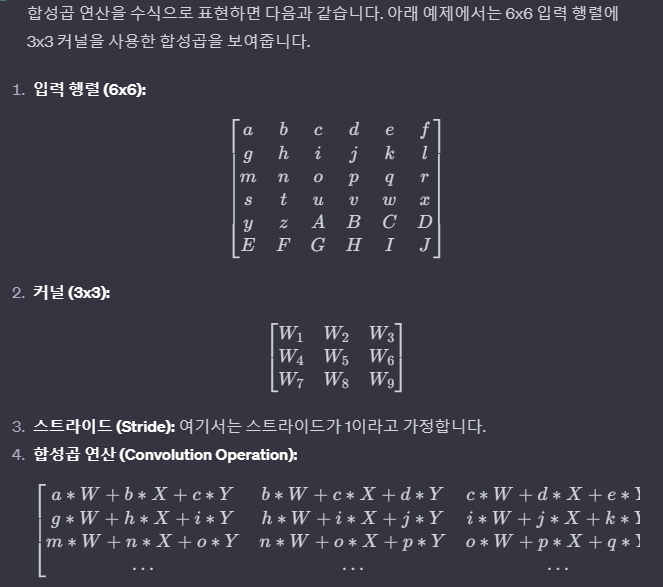
합성곱 신경망(CNN, Convolutional neural network)란 시각적 영상을 분석하는 데 사용되는 다층의 피드-포워드적인 인공신경망의 한 종류이다. 필터링 기법을 인공신경망에 적용하여 이미지를 효과적으로 처리할 수 있는 심층 신경망 기법으로 행렬로 표현된 필터의 각 요소가 데이터 처리에 적합하도록 자동으로 학습되는 과정을 통해 이미지를 분류하는 기법

데이터를 불러오기
mnist = tf.keras.datasets.fashion_mnist
(x_train, y_train), (x_test, y_test) = mnist.load_data()
# 색상채널 추가(흑백)
x_train = x_train.reshape((60000, 28, 28, 1)) # 흑백은 1, RGB는 3
x_test = x_test.reshape((10000, 28, 28, 1)) # 흑백은 1, RGB는 3

# 스케일링
x_train, x_test = x_train/255.0, x_test/255.0
RGB데이터가 있는 이미지라면 색상채널 추가하는 과정은 필요없다. 왜냐하면 색깔은 빛의 3원색의 조화로 생성되기 때문에, 3개의 층에서 각 삼원색의 0~255의 수치가 있을 것이다. 지금은 흑백 데이터 채널을 강제적으로 추가한 것이다.
from tensorflow.keras.layers import Flatten, Dense, Dropout, Conv2D, MaxPooling2D
from tensorflow.keras.models import Sequential

model = Sequential([
                    Conv2D(32, (3, 3), activation='relu', input_shape=(28, 28, 1)),
                    MaxPooling2D((2, 2)),
                    Conv2D(64, (3, 3), activation='relu'),
                    MaxPooling2D((2, 2)),
                    Conv2D(64, (3, 3), activation='relu'),
                    MaxPooling2D((2, 2)),
                    Flatten(),
                    Dense(64, activation='relu'),
                    Dense(10, activation='softmax')
])

model.compile(optimizer='adam',
              loss='sparse_categorical_crossentropy',
              metrics=['accuracy'])
Conv2D-MaxPooling2D의 과정을 3번 거친다. 해당 작업의 결과는 아래와 같다.
model.summary()
epochs를 10회 진행해보겠다.
history = model.fit(x_train, y_train, validation_data=(x_test, y_test), epochs=10)
시각화를 해보자(과적합을 피하고자 val_accuracy도 추가해본다)
plt.plot(history.history['accuracy'], label='accuracy')
plt.plot(history.history['val_accuracy'], label='val_accuracy')
plt.xlabel('epochs')
plt.ylabel('accuracy')
plt.legend()
이번엔 손실함수도 시각화 해보자(과적합을 피하고자 val_loss도 함께 추가해본다)
plt.plot(history.history['loss'], label='loss')
plt.plot(history.history['val_loss'], label='val_loss')
plt.xlabel('epochs')
plt.ylabel('loss')
plt.legend()
해당 지표들을 통해 epochs 횟수를 잘 조절해본다.